Distribution is a most commonly used concept in research and acquaints with the shape of the data. Most of the time when a researcher collects data, S/he wants to know about the characteristics of the study sample. Let’s say, an investigator is interested to know the cancer site of first 1000 patients diagnosed in a tertiary care hospital in a specified year. S/he would just select 1000 patients, gather information from the lab about the diagnosis, and summarize data. These data might give statistics such as the average age, gender, eating habit, smoking pattern, number of breast cancer cases and so on. All of these statistics simply describe characteristics of the sample and are therefore called descriptive statistics. The probability distributions are the part of descriptive statistics to describe the shape of the data and possibly predict the probability of an event.

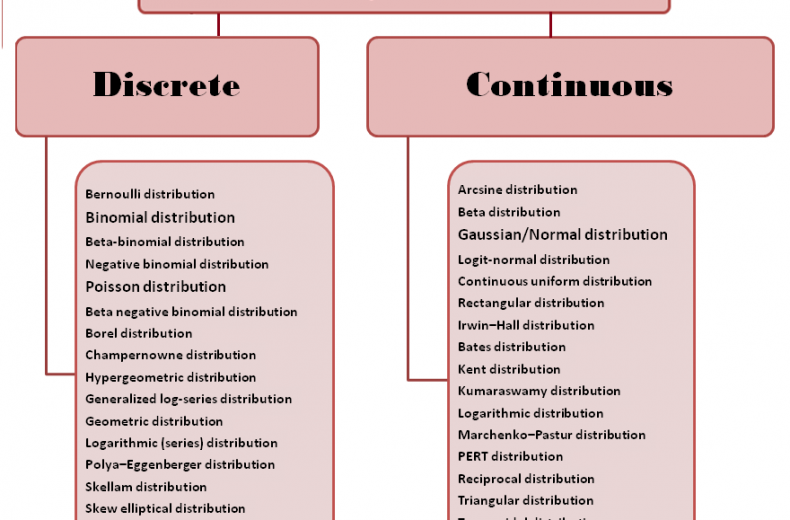
Although there is a number of probability distributions as shown in the figure, majorly three distributions are used in medical research studies i.e. Binomial, Poisson and Gaussian/Normal distribution.

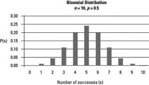Binomial distribution has very wide application and it is important as it allows us to deal with the outcome belongs to two categories such as accepted/rejected, yes/no or male/female. It is a probability model for a discrete outcome with dichotomous nature. It gives you the probability of m successes among n trials of any event. For example, there are 40 kidney cancer patients and we are looking for 5-year survival of 16 patients. The individual patient outcomes are independent and if we assume that the probability of survival is p = 0.20 or 20% for all patients then the required probability will be 0.2%.

Similarly, you may find several options such as what is the probability of at least 16 patients survives, more than 16 patients survives etc.

Poisson distribution describes the behaviour of rare events (with small probabilities) such as patients arriving at an emergency room, decaying radioactive atoms, bank customers coming to their bank, number of suicide cases in adolescence. Let us say your local hospital registered a mean of 2.3 patients arriving at the emergency department on Saturday second half. You can find the probability of exactly four patients arrives on a randomly selected Saturday’s second half.

Another example is taken from CDC. It says 19.3% of adults smoke cigarettes. In 2008, the incidence rate of lung cancer was 65.1 cases per 100,000 people per year. Suppose you are conducting a lung cancer study, and obtain a random sample of 2,000 adults who do not have lung cancer. You plan to follow this study cohort over a period of 5 years and observe incident cases of lung cancer. Considering lung cancer is a rare disease, you can model cases of lung cancer using the Poisson distribution, with incidence rate 65.1 cases per 100,000 person-years. A probability of more than 1 lung cancer case in the first year will be 37.4%.

Or what is the expected number of lung cancer cases observed over the five year study period?

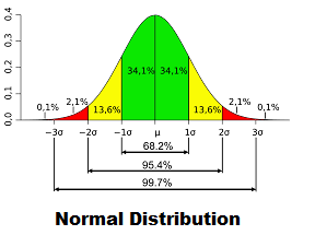The most important continuous probability distribution is the Gaussian or Normal Distribution. It is a bell-shaped slider and also known as symmetrical distribution. The normal distribution has some very nice properties. If two random variables have a normal distribution, their sum has a normal distribution. In general, all kinds of sums and differences of normal variables have normal distributions.

The normal distribution has only two parameters, the mean and the standard deviation (SD). By definition, about 67% of the values of a normal distribution is within ±1 SD of the mean, and about 95% are within ± 2 SDs. Skewed distributions (non-normal) are not appropriately described with the mean and the SD. The median and the interquartile range are more appropriate for describing non-normally distributed data as most of the time biological data is not normally distributed. Also arithmetic mean should not be used to average normalized numbers. In this case, the geometric mean is the right statistics to average normalized numbers.

Almost 90% statistical inference is based on normal distribution. There are hundreds of statistical tests, and tests will not give accurate results if their assumptions are not met. All parametric tests have an assumption of normally distributed data. So the most common application of normal distribution is to identify whether to select a parametric test or non-parametric test. There are many ways to identify whether data is normally distributed such as histogram, box-plot, outliers, normal quantile plot, Shapiro-Wilk test etc. However, most of the statistician assume data to be normal if SD is less than half of the mean.

Other applications of a normal distribution are to find probabilities from given values of a random variable and to find cut-off values of a random variable from a given probability. The entire theory of linear regression is based on the assumption of normality.

Last modified: 21/11/2019